Conditioned choropleth maps

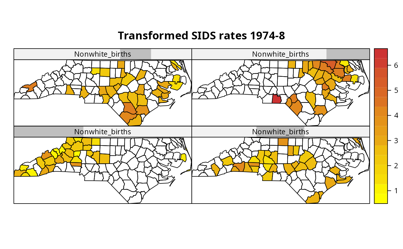
Conditioned choropleth maps permit the conditioning of a map of a variable on the values of one or two other variables coded as factors or shingles. This function uses spplot after constructing multiple subsets of the variable of interest defined by the intervals given by the conditioning variables.

CCmaps(obj, zcol = NULL, cvar = NULL, cvar.names = NULL, ..., names.attr,
 scales = list(draw = FALSE), xlab = NULL, ylab = NULL,
 aspect = mapasp(obj, xlim, ylim), sp.layout = NULL, xlim = bbox(obj)[1, ],
 ylim = bbox(obj)[2, ])

Arguments

obj

object of class SpatialPolygonsDataFrame

zcol

single variable name as string

cvar

a list of one or two conditioning variables, which should be of class factor or shingle

cvar.names

names for conditioning variables, if not given, the names of the variables in the cvar list

...

other arguments passed to spplot and levelplot

names.attr

names to use in panel, if different from zcol names

scales

scales argument to be passed to Lattice plots; use list(draw = TRUE) to draw axes scales

xlab

label for x-axis

ylab

label for y-axis

aspect

aspect ratio for spatial axes; defaults to "iso" (one unit on the x-axis equals one unit on the y-axis) but may be set to more suitable values if the data are e.g. if coordinates are latitude/longitude

sp.layout

NULL or list; see spplot

xlim

numeric; x-axis limits

ylim

numeric; y-axis limits

Value

The function returns a SpatialPolygonsDataFrame object with the zcol variable and the partitions of the cvars list variables invisibly.

References

Carr D, Wallin J, Carr D (2000) Two new templates for epidemiology applications: linked micromap plots and conditioned choropleth maps. Statistics in Medicine 19(17-18): 2521-2538 Carr D, White D, MacEachren A (2005) Conditioned choropleth maps and hypothesis generation. Annals of the Association of American Geographers 95(1): 32-53 Friendly M (2007) A.-M. Guerry's Moral Statistics of France: challenges for multivariable spatial analysis. Statistical Science 22(3): 368-399

Author

Roger Bivand

See also

spplot

Examples

nc.sids <- readShapeSpatial(system.file("shapes/sids.shp",
 package="maptools")[1], IDvar="FIPSNO",
 proj4string=CRS("+proj=longlat +ellps=clrk66"))
#> Warning: shapelib support is provided by GDAL through the sf and terra packages among others
#> Warning: shapelib support is provided by GDAL through the sf and terra paackages among others
#> Warning: shapelib support is provided by GDAL through the sf and terra packages among others
nc.sids$ft.SID74 <- sqrt(1000)*(sqrt(nc.sids$SID74/nc.sids$BIR74) +
 sqrt((nc.sids$SID74+1)/nc.sids$BIR74))
nc.sids$ft.NWBIR74 <- sqrt(1000)*(sqrt(nc.sids$NWBIR74/nc.sids$BIR74) +
 sqrt((nc.sids$NWBIR74+1)/nc.sids$BIR74))
library(lattice)
sh_nw4 <- equal.count(nc.sids$ft.NWBIR74, number=4, overlap=1/5)
CCmaps(nc.sids, "ft.SID74", list("Nonwhite_births"=sh_nw4),
 col.regions=colorRampPalette(c("yellow1", "brown3"))(20),
 main="Transformed SIDS rates 1974-8")